#Install these packages if not already installed
install.packages(c("topicmodels", "stm", "tidytext", "reshape2"))Topic Modeling
Session 3c
1 Latent Dirichelet Allocation (LDA)
Imagine you have a huge pile of documents, and you want to understand what topics they cover without reading each one. This is where topic modeling comes in. Latent Dirichlet Allocation (LDA) is a vanilla topic modeling approach helps you discover the hidden topics in a collection of documents.
1.1 Process of implementing a LDA in R
In general, three main steps are involved with carrying out a topic model after you’ve selected the topic model (e.g., LDA, correlated topic models, structural topic models) to answer your research questions:
- Prepare your data and present them in Document-Feature Matrix (DFM)
- Find a suitable K number of topics based on statistical fit and content
- Inspect, label and visualize the topic
In the following, I will follow these steps to show how to conduct LDA in R. Let’s load the R packages first.
library(quanteda)
library(topicmodels) # for LDA and CTM
library(stm) # for STM
library(sotu)
library(tidyverse)
library(tidytext)
library(reshape2) # helps to run tidytext
2 Prepare SOTU text data and present it in DFM
As a unsupervised learning of text, LDA assumes that each document is a mixture of various topics, and each topic is like a basket of words. For example, a topic about “sports” might have words like “football,” “basketball,” and “athlete,” while a topic about “politics” might have words like “government,” “election,” and “policy.” That is, LDA follows the “bag of words” approach that considers each word in a document separately. In this case, we need to first find the DFM of the corpus.
sotu_text <-sotu_text
sotu_meta <-sotu_meta

# Create a corpus
sotu_corpus <- corpus(sotu_text,
                      docvars=sotu_meta)

# Create tokens with preprocessing
sotu_toks_clean <- sotu_corpus %>%
  tokens(remove_punct = TRUE,
         remove_symbols = TRUE,
         remove_numbers = TRUE
         ) %>%
  tokens_tolower() %>%
  tokens_remove(c(stopwords("en"), "shall", "upon"))

# Create a DFM
sotu_dfm <- dfm(sotu_toks_clean)
I also trim the dfm for sparsity. Here, I removed tokens which are rare (appearing in less that 7.5% of all documents, which is 18 out of the 240 documents) and too often (appearing in more than 95% of documents).
# Trim a DFM for sparsity
sotu_dfm.t<-dfm_trim(sotu_dfm,
                     min_docfreq = 0.075,
                     max_docfreq = 0.95,
                     docfreq_type = "prop")

# the sparsity was reduced to 0.75 from 0.95
sparsity(sotu_dfm)
[1] 0.9411624sparsity(sotu_dfm.t)[1] 0.75249652.1 Convert DFM to DTM for topicmodels
We are almost ready to run the LDA model using the topicmodels package. However, we can’t directly feed the quanteda presented dfm object into the LDA() function from topicmodels. This is because these packages have different ways of representing and processing that data.
In topicmodels, the counterpart of DFM is the Document-Term Matrix (DTM). A DTM is very similar to a DFM - it also has documents as rows and unique words as columns. The main difference is in how the packages expect the data to be organized and formatted.
To proceed with the lda() function from the topicmodels package, we need convert the quanteda presented dfm object to the dtm object.
sotu_dtm <- convert(sotu_dfm.t, to = "topicmodels")3 Fit LDA model
Let’s estimate a LDA model!
Fitted models
Since running the topic models may take some time, depending on your machine’s configuration and resources, I provide the fitted model here for teaching purposes. In the class, you can either fit the model or use the load function to import the fitted models for the subsequent analysis.
set.seed(2024) #setting an arbitrary seed number to ensure that the following lda fitting is reproducible.

sotu_lda_t10<- LDA(sotu_dtm,
                   k = 10, # setting the number of topics
                   method = "VEM" # another option is "Gibbs"
                   )
In LDA, Variational Expectation-Maximization (VEM) and Gibbs sampling are two algorithms often used to estimate the topic assignments for each word in each document. At the end of this R session, I provide a note briefly introducing VEM and Gibbs sampling.
In the LDA() function, the default method is VEM. In practice, the choice between VEM and Gibbs sampling depends on the size of the dataset, the available computational resources, and the desired balance between speed and accuracy.
If you have a large dataset and need faster results, VEM might be a good choice. If you have a smaller dataset or want a more accurate estimate of the topic assignments, and don’t mind the longer runtime, Gibbs sampling could be a better option.
4 Inspecting LDA Results
As introduced on our Monday lecture, LDA produces two important matrices: the document-topic matrix and the topic-word matrix.
4.1 Inspect the document-topic matrix
The document-topic matrix is often referred as “theta (θ)” as the parameter presented in the LDA graphical model. In this matrix, each row corresponds to a document and each column corresponds to a topic. The values in the matrix represent the probability of each topic in each document.

We use the posterior() function from the topicmodels package to extract the document-topic distributions (theta) and convert it into a data frame. In this way, we can further use the tidyverse framework that you are very familiar with to wrangle and inspect the theta matrix.
options(scipen=999) # This line helps turn off the scientific notation

theta_t10 <- posterior(sotu_lda_t10)$topics %>%
  as.data.frame() %>% # converting the theta matrix to a data frame
  rename_with(~ paste0("topic_", .), .cols = seq_along(.)) %>% # adding a common prefix "topic_" to the columns
  mutate(document = row_number())

glimpse(theta_t10)
Rows: 240
Columns: 11
$ topic_1 <dbl> 0.9989074, 0.9991337, 0.9994817, 0.9640571, 0.8939911, 0.6914…
$ topic_2 <dbl> 0.00012139493, 0.00009626084, 0.00005759345, 0.00006175247, 0…
$ topic_3 <dbl> 0.00012139493, 0.00009626084, 0.00005759345, 0.00006175247, 0…
$ topic_4 <dbl> 0.00012139493, 0.00009626084, 0.00005759345, 0.00006175247, 0…
$ topic_5 <dbl> 0.00012139493, 0.00009626084, 0.00005759345, 0.00006175247, 0…
$ topic_6 <dbl> 0.00012139493, 0.00009626084, 0.00005759345, 0.03544883939, 0…
$ topic_7 <dbl> 0.00012139493, 0.00009626084, 0.00005759345, 0.00006175247, 0…
$ topic_8 <dbl> 0.00012139493, 0.00009626084, 0.00005759345, 0.00006175247, 0…
$ topic_9 <dbl> 0.00012139493, 0.00009626084, 0.00005759345, 0.00006175247, 0…
$ topic_10 <dbl> 0.00012139493, 0.00009626084, 0.00005759345, 0.00006175247, 0…
$ document <int> 1, 2, 3, 4, 5, 6, 7, 8, 9, 10, 11, 12, 13, 14, 15, 16, 17, 18…4.1.1 View the top topics for each document
We can view the most relevant topics for each document based on their probabilities. The following codes show how to find the top 5 most probable topics for each document. You can set for other numbers.
top5_topics_t10 <- theta_t10 %>%
  # reshaping the dataframe from a wide format to a long format
  gather(key = "topic", # the new column
         value = "probability", # the value assigned to the new column is the corresponding probability
         -document # reshape all columns except "document"
         ) %>%
  # keep the top 5 most probable topics for each document.
  group_by(document) %>%
  top_n(5, probability) %>%
  ungroup()

head(top5_topics_t10)
# A tibble: 6 × 3
document topic probability
<int> <chr> <dbl>
1 1 topic_1 0.999
2 2 topic_1 0.999
3 3 topic_1 0.999
4 4 topic_1 0.964
5 5 topic_1 0.894
6 6 topic_1 0.691The resulting top5_topics_t10 dataframe can be further used for visualization, summarization, or any other downstream analysis tasks.
The following chunk offer one visualization possibility using heatmap. In this heatmap, each row represents a document, each column represents a topic, and the cell values represent the probabilities (theta values). This visualization helps identify patterns and clusters of documents with similar topic distributions.
theta_t10 %>%
  gather(key = "topic", value = "probability", -document) %>%
  mutate(topic = factor(topic, levels = paste0("topic_", 1:10)),
         document = factor(document, levels = unique(document))) %>%
  ggplot(aes(x = topic, y = document, fill = probability)) +
  geom_tile() +
  scale_fill_gradient(low = "white", high = "steelblue") +
  scale_y_discrete(breaks = function(x) x[seq(1, length(x), by = 20)]) +
  theme_minimal() +
  theme(axis.text.x = element_text(angle = 45, hjust = 1),
        axis.text.y = element_text(size = 8),
        panel.grid.major = element_blank(),
        panel.grid.minor = element_blank()) +
  labs(x = "Topic", y = "Document", fill = "Probability")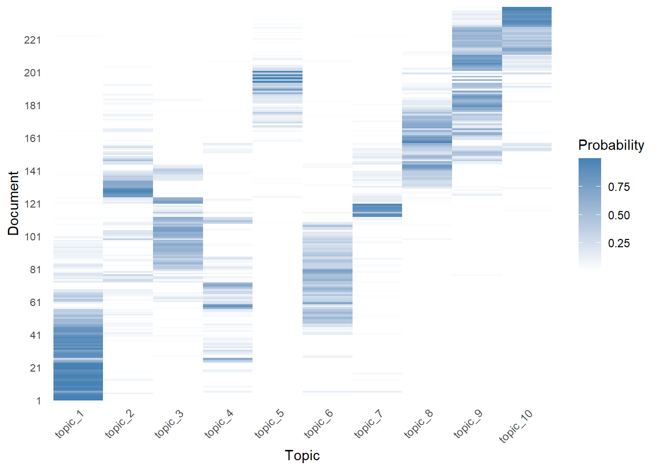
4.2 Inspect the topic-word matrix
The topic-word matrix represents the probability of each word in each topic. This matrix is normally referred as “beta (\(\beta\))”.

You can access beta using the tidy() function from the tidytext package.
beta_t10 <- sotu_lda_t10 %>%
  tidytext::tidy(matrix = "beta")

head(beta_t10, 10)
# A tibble: 10 × 3
topic term beta
<int> <chr> <dbl>
1 1 fellow-citizens 3.82e- 4
2 2 fellow-citizens 2.09e-11
3 3 fellow-citizens 1.18e-13
4 4 fellow-citizens 1.18e- 4
5 5 fellow-citizens 2.89e-60
6 6 fellow-citizens 7.37e- 4
7 7 fellow-citizens 9.71e- 5
8 8 fellow-citizens 2.38e-47
9 9 fellow-citizens 4.87e-46
10 10 fellow-citizens 5.26e-304.2.1 View the most important words for each topic
We can further sort the beta values in each topic to find the corresponding most important words.
# let's see the top 10 most words for each topic
top10_words_beta_t10 <-beta_t10 %>%
  group_by(topic) %>%
  top_n(10, beta) %>%
  ungroup() %>%
  arrange(topic, -beta)

head(top10_words_beta_t10)
# A tibble: 6 × 3
topic term beta
<int> <chr> <dbl>
1 1 present 0.00468
2 1 subject 0.00430
3 1 citizens 0.00414
4 1 general 0.00403
5 1 commerce 0.00401
6 1 part 0.00398We can further use a bar chart to get an idea of the topics by reading their corresponding most important words. In this bar chart, each group represents a topic and each bar within the group represents a top word. We also can compare the relative importance of words across topics. The height of each bar indicates the beta value (importance) of the word within the topic.
top10_words_beta_t10 %>%
  mutate(term = tidytext::reorder_within(term, beta, topic)) %>%
  ggplot(aes(x = beta, y = term, fill = factor(topic))) +
  geom_col(show.legend = FALSE) +
  facet_wrap(~ topic, scales = "free_y") +
  tidytext::scale_y_reordered() +
  labs(x = "Beta (Importance)", y = "Top 10 Words") +
  theme_minimal()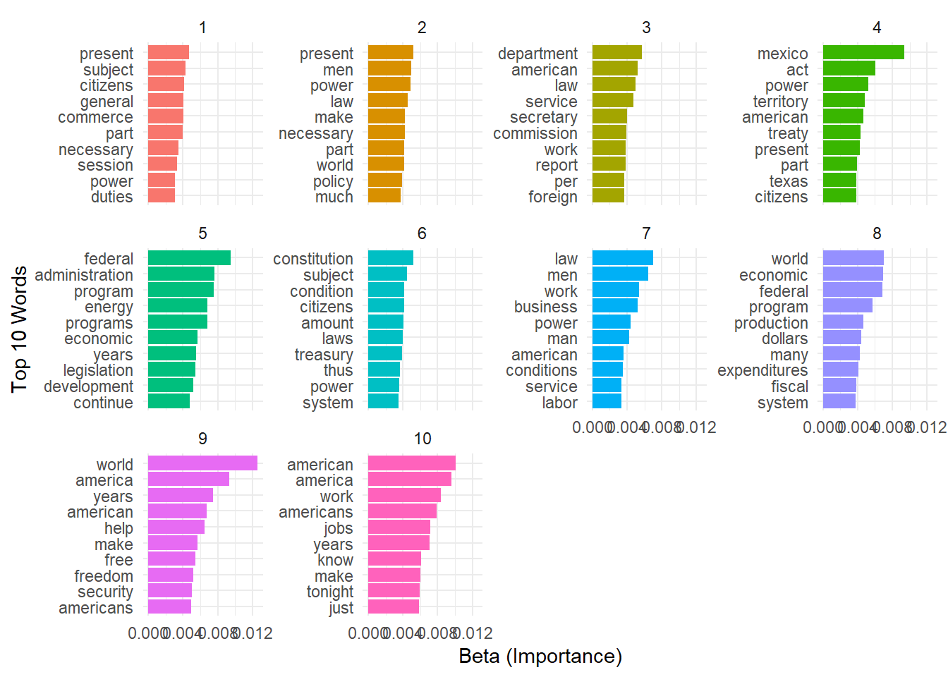
5 Selecting the number of topics
One important decision in using LDA is choosing the number of topics to discover. This is like deciding how many different baskets you want to sort your words into. Too few topics might not capture all the important themes, while too many topics might make the results hard to interpret. In other words, the topic number K controls granularity of topics.
There are a few ways to choose the number of topics:
You can use your own knowledge of the documents to make an educated guess to get started. This is what we did above.
You can try different numbers of topics and see which one gives the most meaningful and interpretable results.
You can use mathematical methods that automatically find the best number of topics based on how well the model fits the data. This selection is based on some model fitness measures.
In practice, it’s often a good idea to try a few different numbers of topics and compare the model selection metrics. Interpretability is equally important, we compare the results to see which one makes the most sense for the particular collection of documents.
Here I show the codes for the mathematical way to find the best number of K. This process requires to load the ldatuning package.
# install.packages("ldatuning")
library(ldatuning)

# You might want to try this code after the class since it will take time
determine_k_lda <- FindTopicsNumber(
  sotu_dtm,
  topics = seq(from = 2, to = 30, by = 1),
  metrics = c("Griffiths2004", "CaoJuan2009", "Arun2010", "Deveaud2014"),
  method = "Gibbs",
  control = list(seed = 77),
  mc.cores = 16L,
  verbose = TRUE
)

FindTopicsNumber_plot(determine_k_lda)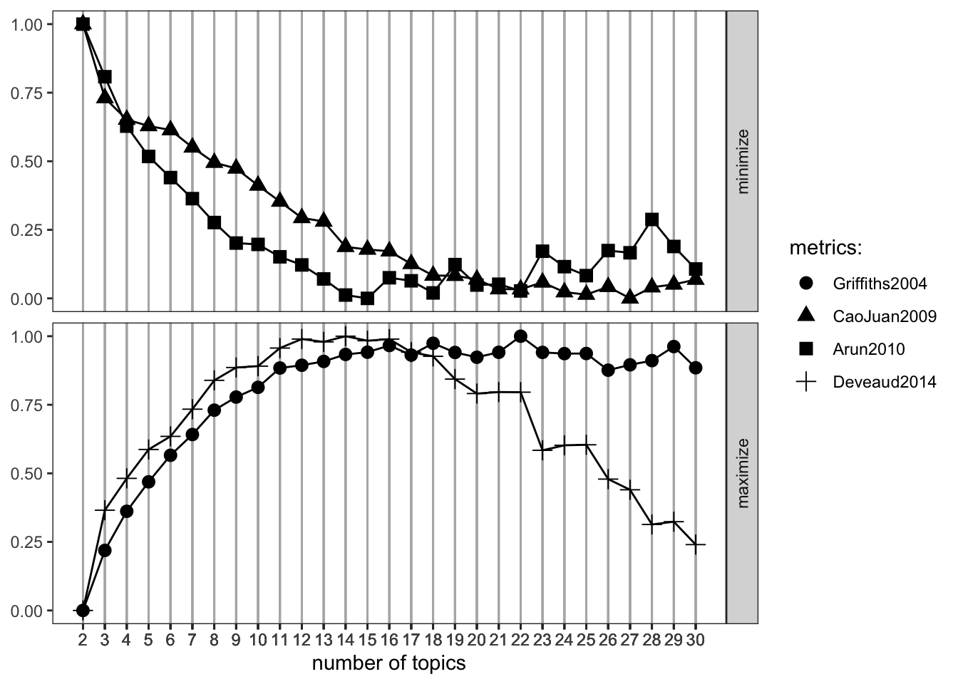
Based on the findings shown from the model selection metrics, the best K could be16, as it maximizes the metrics that shall be maximized and minimizes the other ones quite well. To learn more about these selection metrics, you can start with reading the ldatuning vignette.
At this stage, you can run a K=16 model to inspect the outputs and sense-making the topic themes as we went through above.
6 Structural Topic Modeling:
Structural Topic Modeling (STM) is an extension of LDA that allows for the incorporation of document-level metadata, such as the party and year variables in sotu, into the topic modeling process. STM enables researchers to examine how topic prevalence and content vary with these variables, providing a more nuanced understanding of the underlying themes in a corpus.

6.1 A quick example
We here show a very basic example of running STM using stm package. For a comprehensive guide on conducting STM analysis, refer to the STM website, which provides lists of resources help you learn STM. The vignette provides detailed explanations and examples of how to examine topic prevalence variations across contexts and how words within the same topic are used differently across contexts. It also covers advanced topics such as model selection, convergence checks, and interpreting the results.
6.1.1 Fit STM model
Similar to the conduction of LDA, we first need to convert the dfm object from quanteda to the STM format.
sotu_dfm.stm <- convert(sotu_dfm.t, to = "stm")
names(sotu_dfm.stm)
[1] "documents" "vocab" "meta" You can access the metadata, which is used for providing the contextual variables. The $meta component of the sotu_dfm.stm object contains the document-level metadata associated with the corpus.
head(sotu_dfm.stm$meta) X president year years_active party sotu_type
1 1 George Washington 1790 1789-1793 Nonpartisan speech
2 2 George Washington 1790 1789-1793 Nonpartisan speech
3 3 George Washington 1791 1789-1793 Nonpartisan speech
4 4 George Washington 1792 1789-1793 Nonpartisan speech
5 5 George Washington 1793 1793-1797 Nonpartisan speech
6 6 George Washington 1794 1793-1797 Nonpartisan speechLet’s fit a STM model with K=10 using the stm function from the stm package.
sotu_stm_t10 <- stm(documents=sotu_dfm.stm$documents,
                    vocab=sotu_dfm.stm$vocab,
                    prevalence =~ party+s(year), # specify the covariates you are interested to investigate on topic prevalence.
                    K = 10,
                    data = sotu_dfm.stm$meta,
                    init.type = "Spectral",
                    verbose=FALSE)
6.1.2 Inspect the results
The labelTopics() function is used to generate labels for the extracted topics based on the most prevalent words within each topic. Four different types of word weightings are provided. Check out the details via ?labelTopics
prevalent_words_stm_k10<-labelTopics(sotu_stm_t10,
                                     n=10 # show the top 10 words
                                     )

str(prevalent_words_stm_k10)
List of 5
$ prob : chr [1:10, 1:10] "america" "department" "federal" "present" ...
$ frex : chr [1:10, 1:10] "applause" "silver" "dollars" "objects" ...
$ lift : chr [1:10, 1:10] "applause" "damages" "modest" "persuaded" ...
$ score : chr [1:10, 1:10] "applause" "damages" "modest" "persuaded" ...
$ topicnums: int [1:10] 1 2 3 4 5 6 7 8 9 10
- attr(*, "class")= chr "labelTopics"We can plot the topic porportions.
plot(sotu_stm_t10)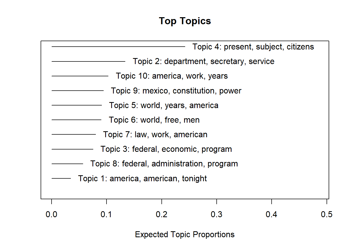
6.1.3 Finding the K
Similar to LDA, STM also requires specifying the number of topics (K) to extract. The searchK() function in the stm package can be used to perform a search for the optimal number of topics based on various metrics, such as held-out likelihood or semantic coherence.
Using one core, the following task of searching a list of Ks takes about 7 minutes.
sotu_stm_searchK <- searchK(documents=sotu_dfm.stm$documents,
        vocab=sotu_dfm.stm$vocab,
        prevalence =~ party+s(year),
        K = c(10,20,30,40,50,60), #specify K to try
        heldout.seed = 2024, # optional
          data = sotu_dfm.stm$meta,
        init.type = "Spectral",
verbose=F)diag.sotu_stm<-plot(sotu_stm_searchK)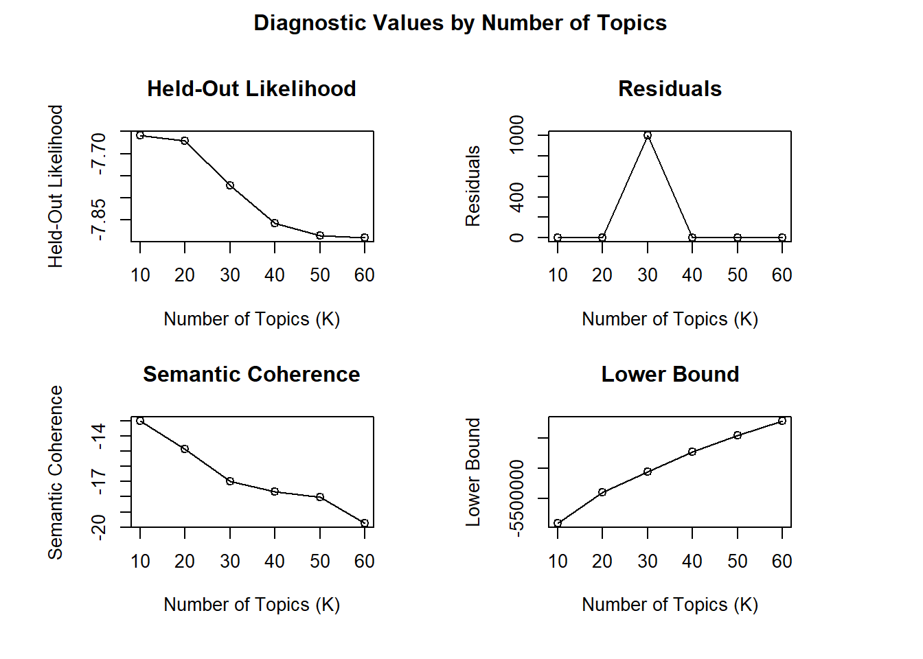
We look for patterns or trends in the diagnostic values:
Identify the point where the held-out likelihood starts to plateau or reaches its maximum.
Find the value of K that maximizes the semantic coherence score.
Check where the residuals start to stabilize or reach a minimum.
Consider the value of K that maximizes the lower bound.
Based on these observations, we can narrow down the range of potential K values to be around 10. Then we can run a few such STMs that strikes a balance between good diagnostic values and interpretable, meaningful topics.
6.1.4 Inspecting topics across contexts
sotu_stm_t10.est <- estimateEffect(formula = 1:10 ~ party+s(year),
                                             stmobj = sotu_stm_t10,
                                   metadata = sotu_dfm.stm$meta,
uncertainty="Global")summary(sotu_stm_t10.est, topics=5)
Call:
estimateEffect(formula = 1:10 ~ party + s(year), stmobj = sotu_stm_t10,
    metadata = sotu_dfm.stm$meta, uncertainty = "Global")


Topic 5:

Coefficients:
                            Estimate Std. Error t value Pr(>|t|)
(Intercept)                -0.001210   0.246011  -0.005   0.9961
partyDemocratic-Republican  0.001447   0.090068   0.016   0.9872
partyFederalist             0.008588   0.144865   0.059   0.9528
partyNonpartisan            0.004473   0.200902   0.022   0.9823
partyRepublican             0.024262   0.029583   0.820   0.4130
partyWhig                  -0.005968   0.062789  -0.095   0.9244
s(year)1                   -0.018066   0.275249  -0.066   0.9477
s(year)2                    0.023916   0.243997   0.098   0.9220
s(year)3                    0.018381   0.274617   0.067   0.9467
s(year)4                   -0.047752   0.252071  -0.189   0.8499
s(year)5                    0.026133   0.258559   0.101   0.9196
s(year)6                   -0.049632   0.257283  -0.193   0.8472
s(year)7                    0.455805   0.267775   1.702   0.0901 .
s(year)8                    0.395357   0.276366   1.431   0.1540
s(year)9                   -0.272281   0.270112  -1.008   0.3145
s(year)10                   0.074044   0.260099   0.285   0.7762
---
Signif. codes: 0 '***' 0.001 '**' 0.01 '*' 0.05 '.' 0.1 ' ' 1plot(sotu_stm_t10.est, covariate = "party", topics = c(5), model = sotu_stm_t10, method = "pointestimate",
main = "Effect of Party on Topic Proportion",
labeltype = "custom",
custom.labels = c("Nonpartisan", "Federalist", "Democratic-Republican", "Democratic", "Whig", "Republican"))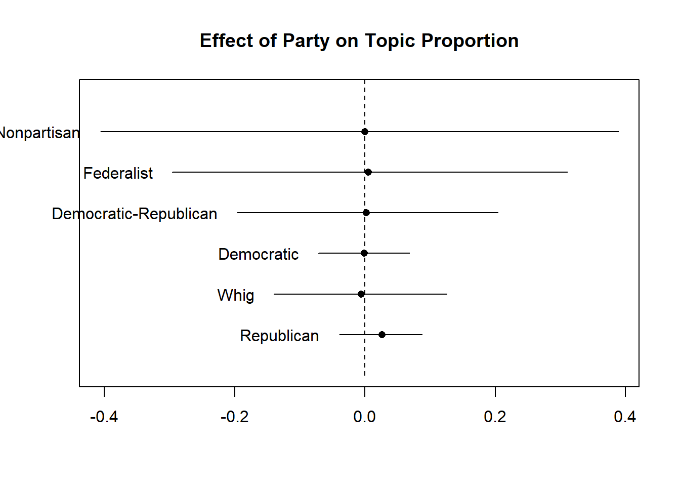
7 Notes
Choosing the estimation method of LDA
VEM is a deterministic algorithm that tries to approximate the true distribution of topic assignments by using a simpler, more tractable distribution. It iteratively updates the parameters of this simpler distribution to make it as close as possible to the true distribution.
On the other hand, Gibbs sampling is a stochastic algorithm that goes through each word in each document and tries to guess which topic basket the word belongs to. It makes this guess based on two things: how often the word appears in the document, and how often the word is associated with each topic basket across all documents
By repeatedly guessing the topic for each word, LDA gradually improves its understanding of the topics and their word baskets. It’s like sorting a big pile of words into different topic baskets, and then adjusting the baskets based on how well the words fit together. After a while, LDA settles on a set of topics and word baskets that best explain the patterns in the documents.
VEM is generally faster than Gibbs sampling, especially for large datasets.Compared to VEM, Gibbs sampling can provide a more accurate estimate of the true distribution of topic assignments, as it doesn’t rely on a simplifying assumption. However, it can be computationally more expensive and may require a longer runtime, especially for large datasets.
You can find a mathematical illustration of LDA estimation in the vignette of topicmodels.